How can we predict how much increase in sales will we get after spending money on different types of ads? I am using Advertising data here to show this and any company can collect this kind of data maybe from different branches and answer the questions: For how much are we going to increase sales spending the curtain amount of money on ads? How much will sales increase when we spend a certain amount of money on ads? Which media, TV, radio or newspaper is effective? I used Linear Regression to answer these questions and according to linear regression formula for our data, if we spend $1000 on TV we increase sales by 19 units plus spending $1000 on radio gives us an additional 29 units plus the synergy effect 1.1 units, total 49 units. If we spend $2000 on both media, we get an increase in sales by about 100 units.

I did this project while I was reading the book ‘An Introduction to Statistical Learning’ and wanted to understand how we can predict sales using our previously collected data and the linear regression formula after we have fitted the model to the data. There is guidance in the book, but the actual code for this data is not given, so I wrote it myself. I wanted to use linear regression because it’s the only method which gives the outcome which is easy to interpret. But in order to use it we need to have data for which the additivity and linearity assumptions hold, otherwise we still use linear regression, but need to transform the data. So, this is what we do before we fit the model to the data, clean it and check if our assumptions hold.

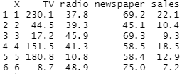
Let’s import the Advertising data and take a look. On the output below we can see that we have 3 predictors: TV, radio, newspaper. The corresponding columns show the amount of money spent on ads for each advertising type. The response variable is sales. All values are in 1000s, for example, the values 10.4 in the second row of the sales’ column is equivalent to 10,400 units sold and 44.5 for TV means $44,500 spent on this media. The sample size is 200, it’s the data collected from two hundred cities.

Advertising <- read.csv("Advertising.csv", head=TRUE)
head(Advertising)

OUTPUT:

We will be answering 7 questions

Question 1: Is there a relationship between advertising and sales?

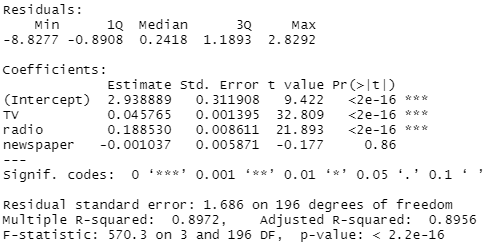
To answer this question, we will then fit the multiple regression model to test the Ho hypothesis. We use F-statistic for this, there is a relationship between the response and predictors when the F-statistic is greater than 1. But how big is big? When the p-value is less than 0.05, we can conclude that there is a relationship. As we can see on the output1 below the p-value(2.2e-16=0.00000000000000022) corresponding to the F-statistic(570.3) is very close to zero, indicating clear evidence of a relationship between advertising and sales.

attach(Advertising)
advertising_fit <- lm(sales ~ TV + radio + newspaper)
summary(advertising_fit)

OUTPUT 1:

Question 2: How strong is the relationship?

We will look at the above output1 and use R-squared statistic(0.8972) to decide. The value of 0.8972 means that the predictors explain almost 90% of the variance in sales, so the relationship is strong.

Question 3: Which media contribute to sales?

To answer this question, we need to examine the p-values associated with each predictor’s t-statistic using again the same output1 above. As we can see, the p-values for TV and radio are low and equal to 2e-16. We can’t state the same about the p-value for newspaper which is 0.86. This suggests that only TV and radio are related to sales.

Question 4: How large is the effect of each medium on sales?

We need to look at the confidence intervals of the coefficients. Looking at the output2 below we can see that for the Advertising data, the 95% confidence intervals are as follows: (0.043, 0.049) for TV (coefficient value=0.046), (0.172, 0.206) for radio (0.189), and (−0.013, 0.011) for newspaper (-0.001). The confidence intervals for TV and radio are narrow and far from zero, providing evidence that these media are related to sales. But the interval for newspaper includes zero, indicating that the variable is not statistically significant given the values of TV and radio.

confint(advertising_fit)

OUTPUT 2:

We will examine this further to see if collinearity be the reason that the confidence interval associated with newspaper is so wide? As a rule of thumb, a VIF value that is bigger than 5 or 10 indicates a problematic of collinearity. From the output 3 we can see that the VIF scores are 1.005, 1.145, and 1.145 for TV, radio, and newspaper, suggesting no evidence of collinearity.

library(car)
vif(advertising_fit)

OUTPUT 3:

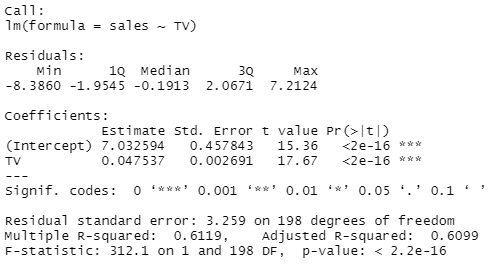
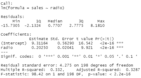
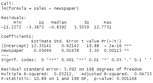
In order to assess how large is the effect of each medium individually on sales, we can fit three separate simple linear regression models. Results are shown on output4 and output5. There is evidence of an extremely strong association between TV and sales and between radio and sales. There is evidence of a mild association between newspaper and sales (output6), when the values of TV and radio are ignored.

advertising_fit_TV <- lm(sales ~ TV)
advertising_fit_radio <- lm(sales ~ radio)
advertising_fit_newspaper <- lm(sales ~ newspaper)

OUTPUT 4:

OUTPUT 5:

OUTPUT 6:

Question 5: How accurately can we predict future sales?

The response can be predicted using the following formula (this is not our final model and that’s why we will ignore newspaper variable as we have seen that it’s not important)

sales = 2.94 + 0.05 x TV + 0.19 x radio + e

The accuracy associated with this estimate depends on whether we wish to predict an individual response (for a particular city out of our 200 cities), or the average response (over a large number of cities). If the former, we use a prediction interval, and if the latter, we use a confidence interval. As we can see on the output7, prediction intervals are wider than confidence intervals and this will always be the case because they account for the uncertainty associated with e, the irreducible error.

newdata=data.frame(TV = 1, radio = 1, newspaper = 1)
predict(advertising_fit, newdata, interval = 'prediction')
predict(advertising_fit, newdata, interval = 'confidence')

OUTPUT 7:

Question 6: Is the relationship linear?

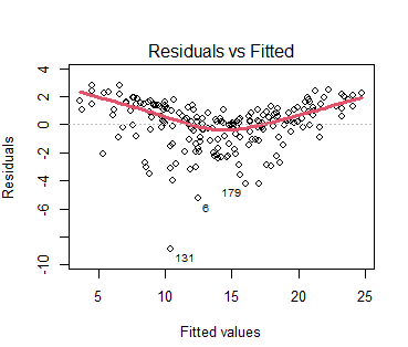
The residual plots can be used in order to identify non-linearity. If the relationships are linear, then the residual plots should display no pattern. We will look only at the plot of residulas vs. predicted (of fitted) values. U-shape we can see on output8 below provides evidence of non-linearity. We can use non-linear transformations of the predictors, such as log X, square root of X, and X squared, in the linear regression model in order to accommodate non-linear relationships.

par(mfrow=c(2,2))
plot(advertising_fit, lwd=3)

OUTPUT 8:

Question 7: Is there synergy among the advertising media?

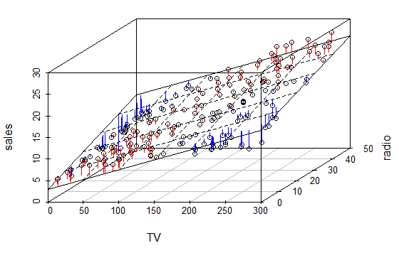
The standard linear regression model assumes an additive relationship between the predictors and the response, meaning that the effect of changes in one of the predictors (let’s say money spent on TV ads) on the response (sales) is independent of the values of the other predictors (radio and newspaper). An additive model is easy to interpret. However, the additive assumption may be unrealistic for certain data sets. Output9 suggested that the Advertising data may not be additive. We see that some observations lie above and some observations lie below the least squares regression plane. In particular, the linear model seems to overestimate sales for instances in which most of the advertising money was spent exclusively on either TV or radio. It underestimates sales for instances where the budget was split between the two media. This pronounced non-linear pattern cannot be modeled accurately using linear regression. It suggests a synergy(phenomenon known in business) or interaction effect(term used in statistics) between the advertising media, whereby combining the media together results in a bigger boost to sales than using any single media. Very interesting insight to know!

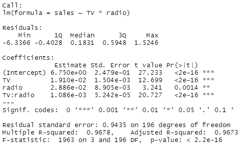
A small p-value (output10) associated with the interaction term indicates the presence of such relationships. Including an interaction term in the model results in a substantial increase in R-squared, from around 90% to almost 97%!

OUTPUT 9:

advertising_fit_int <- lm(sales ~ TV * radio)
summary(advertising_fit_int)

OUTPUT 10:

We have properly fitted the multiple linear regression model with the interaction term to the data, we can make predictions using the following formula.

sales = 6.75 + 0.0191 x TV + 0.0289 x radio +  0.0011 x TV x radio + e

The interaction term makes our predictions a little bit more trickier but still easy. Because the data is 1000s, we use this instead of 1 when predicting. According to our linear regression formula, if we spend $1000 on TV we increase sales by 19 units plus spending $1000 on radio gives us an additional 29 units plus the synergy effect 1.1 units, total 49 units. If we spend $2000 on both media, we get an increase in sales by about 100 units. The output11 and output12 show total sales, not just increase in sales as we were already selling 6,750 units and now we will be selling 6,850 units, 100 more. Also, we are more confident about this value of 6.85 for all 200 cities where the confidence intervals are (6.396, 7.305) than for the particular city where the prediction intervals are (4.935, 8.766).

# prediction intervals(1 city) and confidence intervals (all 200 cities)
newdata1=data.frame(TV = 1, radio = 1)
predict(advertising_fit_int, newdata1, interval = 'prediction')
predict(advertising_fit_int, newdata1, interval = 'confidence')

OUTPUT 11:

# prediction intervals(1 city) and confidence intervals (all 200 cities)
newdata1=data.frame(TV = 2, radio = 2)
predict(advertising_fit_int, newdata1, interval = 'prediction')
predict(advertising_fit_int, newdata1, interval = 'confidence')

OUTPUT 12:

This kind of information is very useful for a business as now they know how much to spend and on what media to increase sales, not waste money and time anymore.

If I had more time, I would look more at the linearity assumptions and would make some transformations and use LOOCV(Leave-One-Out Cross-Validation) to choose the right model. This would further improve the model performance meaning more accurate predictions.

Photo source: slidebean/Unsplash