The aim of the project was to analyse the outcomes of the experiment held by an agricultural scientist who wanted to compare the effect of weed control on wheat yield. Plus, summarize conclusions for the nontechnical reader. I used ANOVA to analyse data. The optimum treatment combination(cheap and effective) would be potassium level 3 and combination of herbicide sprayed and nitrogen level 1. The average yield mean if applying our optimum treatment will be (6.92 + 9.41 + 8.58)/3 = 8.30 and the average yield mean with no additives will be (1.78 + 1.69 + 1.71)/3 = 1.73, so the difference is 6.57, almost 5 times bigger. What the farmers could do in order to control weed the best and increase the yield is to use herbicide spray and combine it with nitrogen level 1(low) and potassium level 3(high). This way they could get almost five times more yield during the harvest time!
This project was the requirement for my module on Experimental Design for my MSc Statistical Data Science course at the University of Kent. The aim of the project was to analyse the outcomes of the experiment held by an agricultural scientist who wanted to compare the effect of weed control on wheat yield using a herbicide spray regime versus a regime where no spray is used. He also wished to see how this interacts with different fertiliser regimes, consisting of all combinations of 4 nitrogen levels, and 5 potassium levels. The experiment thus has 40 treatment combinations which are applied to 120 plots laid out in three blocks of 40 plots per block. At the end of the season the wheat is harvested and the yield recorded for each plot. The resulting data was a table containing mean values from these 120 plots. One of the tasks on this assessment was to report analysis and include a summary paragraph detailing conclusions for the nontechnical reader.
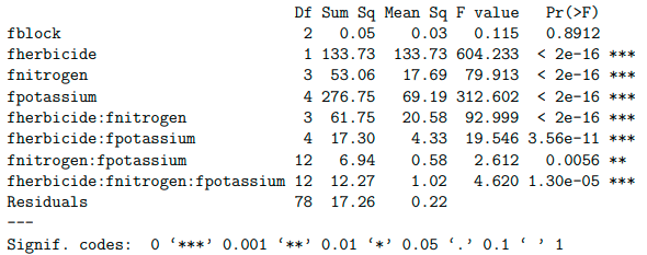
I used ANOVA to analyse data. In order to be able to use this method, we need to check for variance heterogeneity and non-normality and, if detected, take appropriate action. To check our residuals to see that our assumptions on variance homogeneity and normality hold we use R and conduct analysis of variance and look at the plots:
weedcontrol<- read.table("weedcontrol.txt", header=TRUE)
weedcontrol
summary(weedcontrol)

weedcontrol$fblock <- factor(weedcontrol$block)
weedcontrol$fherbicide <- factor(weedcontrol$herbicide)
weedcontrol$fnitrogen <- factor(weedcontrol$nitrogen)
weedcontrol$fpotassium <- factor(weedcontrol$potassium)

aov1 <- aov(yield ~ fblock + fherbicide * fnitrogen * fpotassium,
data=weedcontrol)

summary(aov1)
OUTPUT 1:
par(mfrow=c(2,2))
plot(aov1)
OUTPUT 2:
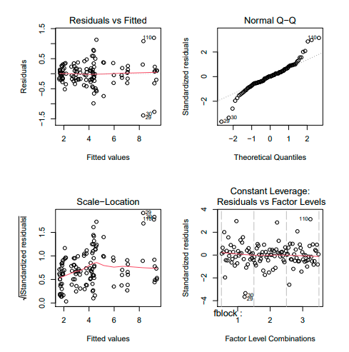
Looking at our top left residual plot and checking we can see the fan shape which means that as mean increases, the variance increases. On our bottom left standardized residuals plot we can see that the line is not horizontal. This means that our variance is not constant. On all four of our plots we can see outliers 29, 30, 110 and looking at our top right QQ plot, we can see that there is something wrong in the tails, suggesting that probably our error doesn’t have a normal distribution. To overcome these problems we need to use a log transform, conduct analysis of variance again and look at the plots. Later we will back transform some values of interest using exp function in R.
weedcontrol$y<-log(weedcontrol$yield)
aov2 <- aov(y ~ fblock + fherbicide * fnitrogen * fpotassium,
data=weedcontrol)

plot(aov2)
OUTPUT 3:
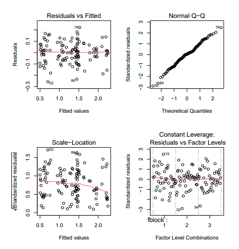
Looking at our new plots(aov2) we can see that the actions we took overcome the problem. On our top left residual plot the fan shape changed, on the left bottom standardized residual plot the red line is closer to the horizontal line and our new top right QQ plot shows that the problem with tails is solved.
We can now move to conducting an ANOVA table and testing for treatment effects.
OUTPUT 4:
aov2 <- aov(y ~ fblock + fherbicide * fnitrogen * fpotassium,
data=weedcontrol)

summary(aov2)
OUTPUT 5:
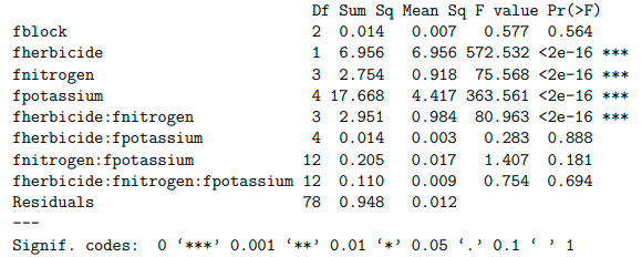
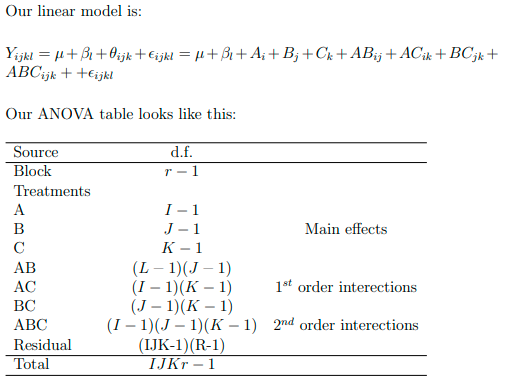
We analysed the outcome using the hierarchical principle. First looked at the second order interaction to see if it’s significant, in our case it’s not, then we move up to the first order interactions, in our case only herbicide with nitrogen interaction is significant, which means that we will look further only at potassium’s main effect. It turns out that potassium’s main effect is significant.
Next, we need to compare treatments to recommend an optimum treatment combination. We will compare means and interpret the results
library(emmeans)
emmeans(aov2, pairwise ~ fherbicide:fnitrogen)
emmeans(aov2, pairwise ~ fpotassium)
$emmeans
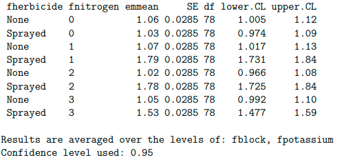
# The components with the higest yield is combination of herbicide (sprayed) and nitrogen level 1 which is 1.79
OUTPUT 6:
$contrasts
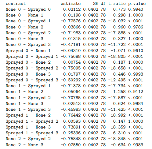
# We can check the means for herbicide and nitrogen combination and see that herbicide sprayed with nitrogen level l doesn’t differ significantly with herbicide sprayed with nitrogen level 2 (t.ratio =-0.147, p.value=1.0000), in this case using level 1 of nitrogen is cheaper
OUTPUT 7:

emmeans(aov2, pairwise ~ fpotassium)
# NOTE: Results may be misleading due to involvement in interactions
$emmeans
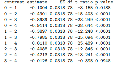
#The components with the higest yield is potassium level 4 which is 1.724.
OUTPUT 8:

$contrasts
# Because from the analysis of contrasts we know that potassium level 3 doesn't differ significantly from level 4 (t.ratio =-0.395, p.value = 0.9948) we can suggest the best treatment level 3 as it is a smaller amount so it’s cheaper!
OUTPUT 9:
Report Our Analysis
Looking at our interaction, second order interaction is not significant, from the first class interactions only herbicide with nitrogen interaction is significant as well as the main effect of potassium. The components with the highest yield are potassium level 4 which is 1.724 and the combination of herbicide (sprayed) and nitrogen level 1 which is 1.79. Because from the analysis of contrasts we know that potassium level 3 don’t differ significantly from level 4 (t.ratio =-0.395, p.value = 0.9948) we can suggest as best treatment level 3 as it is smaller amount so it’s cheaper. The same way we checked the means for herbicide and nitrogen combination and saw that herbicide sprayed with nitrogen level l doesn’t differ significantly with herbicide sprayed with nitrogen level 2 (t.ratio =-0.147, p.value=1.0000), in this case using level 1 of nitrogen is cheaper. So, our optimum treatment combination would be potassium level 3 and combination of herbicide sprayed and nitrogen level 1.
Estimate of the Effect on Yield of Applying the Optimum Treatment Combination When Compared with the Effect of No Additives
To estimate the effect on yield of our optimum treatment we can compare it with the yield when no additives are used. We can do it by comparing means. The average yield mean if applying our optimum treatment will be (6.92 + 9.41 + 8.58)/3 = 8.30 and the average yield mean with no additives will be (1.78 + 1.69 + 1.71)/3 = 1.73, so the difference is 6.57, almost 5 times bigger!
Summary Paragraph on Conclusions for the Nontechnical Reader
What the farmers could do in order to control weed the best and increase the yield is to use herbicide spray and combine it with nitrogen level 1(low) and potassium level 3(high). This way they could get almost five times more yield during the harvest time.
Photo source: chuttersnap/Unsplash