The aim of this project is to forecast the average number of goals for the English Premier League using data for the previous years. I used R programming language to choose the right model, conduct diagnostics and forecast. The data showed the average number of goals is decreasing with time, our model predicted that the average number of goals for the future four years will stay low.
We will need the following packages and libraries
library(forecast)
library(timeDate)
library(timeSeries)
library(fBasics)
library(fGarch)
We will first importing data and remove the first column which is not useful for us
Premierleague_goals <- read.csv("Premierleague_goals.csv", header=FALSE, comment.char="#")[,-1]
head(Premierleague_goals)
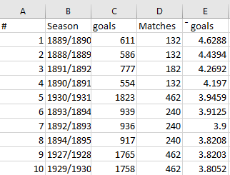
View our data and its ACF plots
par(mfrow=c(3,2))
ts.plot(Premierleague_goals[,2])
acf(Premierleague_goals[,2])
ts.plot(Premierleague_goals[,3])
acf(Premierleague_goals[,3])
ts.plot(Premierleague_goals[,4])
acf(Premierleague_goals[,4])
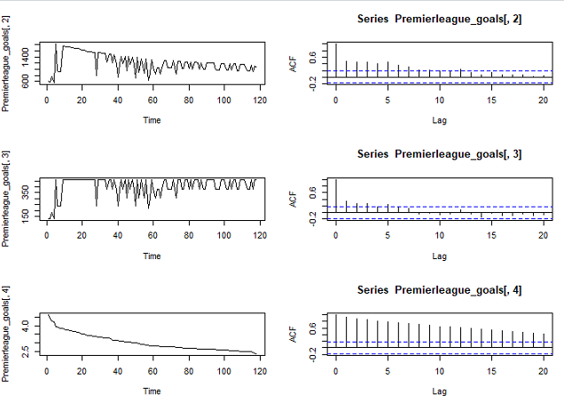
As the ACF for Premierleague_goals[,4] data is decaying linearly, we have evidence of a unit root so we need to difference. The differenced data (the plot below) seem to exhibit more stationary features.
ts.plot(diff(Premierleague_goals[,4]))
acf(diff(Premierleague_goals[,4]))

We will also remove the first 4 observations as they seem a bit out-of-line with the rest of the data and look at the plots
x=diff(Premierleague_goals[,4])
x=x[-(1:4)]
tsdisplay(x)
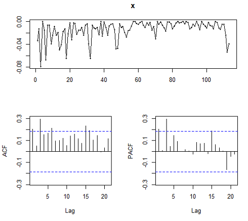
In the plot above we can see that the average number of goals is decreasing with time. The ACF and PACF suggest some spikes of order p = 3, q = 3, we might like to consider those values together with the smaller models so we fit 10 different models. We use arima command which uses Maximum Likelihood Estimation to calculate the coefficients
fit1=arima(x,c(1,0,1))
fit2=arima(x,c(2,0,1))
fit3=arima(x,c(3,0,1))
fit4=arima(x,c(3,0,0))
fit5=arima(x,c(3,0,2))
fit6=arima(x,c(2,0,2))
fit7=arima(x,c(1,0,2))
fit8=arima(x,c(0,0,2))
fit9=arima(x,c(0,0,3))
fit10=arima(x,c(1,0,3))
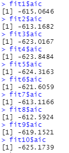
The best model is the one with the smallest AIC. It is observed for model 10: fit10=arima(x,c(1,0,3))
Now we need to perform a model diagnostics for our model by using tsdiag which uses the old Ljung-Box test statistics
tsdiag(fit10)
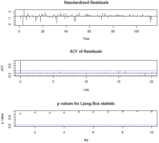
But the best goodness of fit test is Weighted Monti test as it is the most powerful. I know this as this was the topic of my dissertation project for my MSc Statistical Data Science course
install.packages('WeightedPortTest')
library('WeightedPortTest')
Weighted.Box.test(residuals(fit10), lag = 10,
                  type = "Monti",
                  fitdf = 0, weighted = TRUE)

Now when we have the best model, we can forecast for let’s say 4 future Premier League seasons
forecast(fit10, h=4)

Now let’s look at the final plot! The future average goal values are shown by blue spots, grey area is 80% and 95% confidence intervals for the values.
plot(forecast(fit10, h=4))
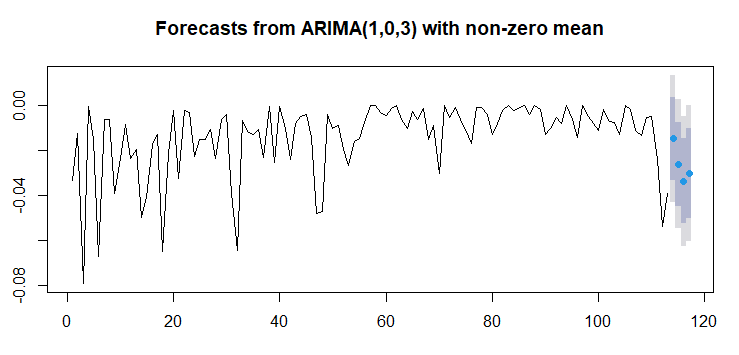
Our Results
We have seen that the average number of goals is decreasing with time, our model predicts that the number will stay low.
Banner photo source: chris_liverani/Unsplash