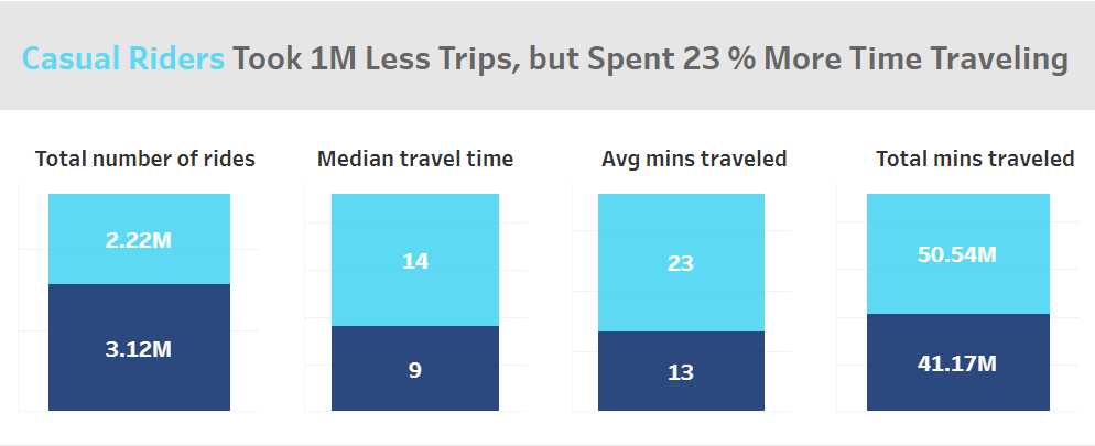
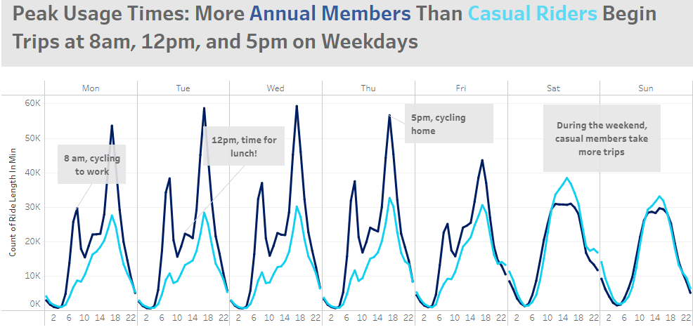
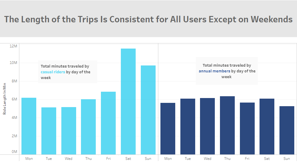
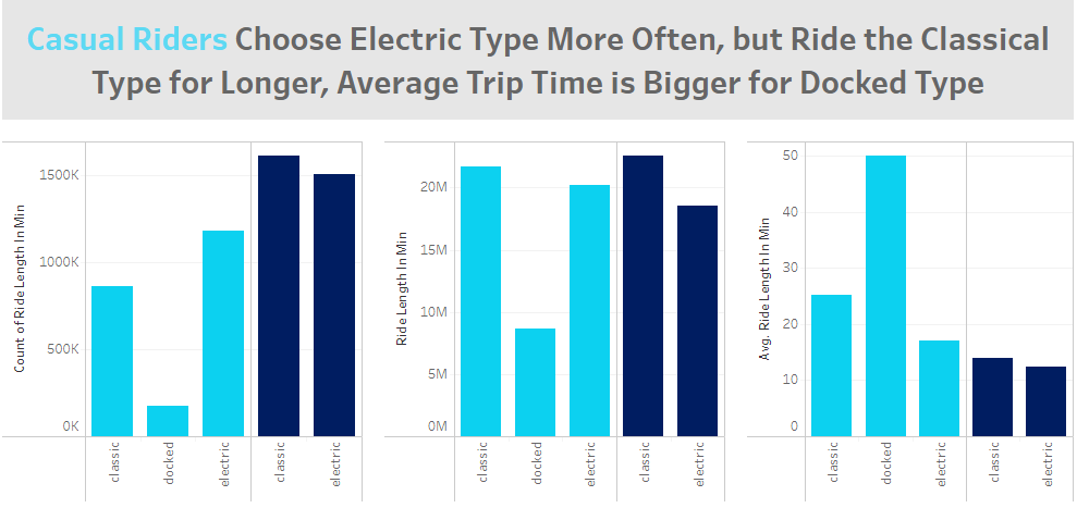
This is a case study I have done in order to obtain my Google Data Analyst Professional Certificate. Scenario: It’s about Cyclistic, a bike-share company in Chicago. There are three types of bikes: classical, electric, and docked. The director of marketing believes the company’s future success depends on maximizing the number of annual memberships. My task was to answer the question “How do annual members and casual riders use Cyclistic bikes differently?” and come up with three recommendations based on my analysis. From these insights, the team will design a new marketing strategy to convert casual riders into annual members. Cyclistic is a fictional company. The data has been made available by Motivate International Inc. I have chosen data from January 2022 to December 2022. I used RStudio for data manupulation and Tableau to conduct the analysis and create visualisations and a dashboard.
Step 1: Importing Data
Data was downloaded from the following link
Importing required packages in RStudio
library(tidyverse)
library(ggplot2)
Load 12 datasets correspoding to 12 months
data1=read.csv("trips_jan_22.csv")
data2=read.csv("trips_feb_22.csv")
data3=read.csv("trips_mar_22.csv")
data4=read.csv("trips_apr_22.csv")
data5=read.csv("trips_may_22.csv")
data6=read.csv("trips_jun_22.csv")
data7=read.csv("trips_jul_22.csv")
data8=read.csv("trips_aug_22.csv")
data9=read.csv("trips_sep_22.csv")
data10=read.csv("trips_oct_22.csv")
data11=read.csv("trips_nov_22.csv")
data12=read.csv("trips_dec_22.csv")
Step 2: Data preparation
Load packages for data manipulation and handling dates and times
library("dplyr")
library(lubridate)
Union 12 months data in one dataset
data=rbind(data1,data2,data3,data4,data5,data6,data7,data8,data9,data10,data11,data12)
View the new data
head(data)
colnames(data)
View(data)
str(data)
class(data$started_at)
class(data$ended_at)
Changing variables started_at_as_date and ended_at_as_date to date type
data$started_at_as_date=dmy_hm(data$started_at)
data$ended_at_as_date=dmy_hm(data$ended_at)

class(data$started_at_as_date)
class(data$ended_at_as_date)
Creating a new variable ride_length_in_min for the ride duration in minutes
data$ride_length_in_min=as.numeric(data$ended_at_as_date-data$started_at_as_date,
                                   units="mins")
Creating a new variable week_day_as_date to see the week day of the start of the trips
data$week_day_as_date=wday(data$started_at_as_date,label=TRUE, abbr=TRUE)
Changing categories of the rideable_type variable to classic, electric, and docked
data=data %>%
  mutate(rideable_type=replace(rideable_type, rideable_type=="classic_bike", "classic"))
data=data %>%
  mutate(rideable_type=replace(rideable_type, rideable_type=="electric_bike", "electric"))
data=data %>%
  mutate(rideable_type=replace(rideable_type, rideable_type=="docked_bike", "docked"))
Load packages for summary statistics, cleaning, and preprocessing data
library(skimr)
library(janitor)
Generating summary statistics
skim_without_charts(data)
data %>%
  group_by(member_casual) %>%
  summarise(mean(ride_length_in_min), min(ride_length_in_min), max(ride_length_in_min))
Filtering data, keeping only ride_length_in_min >= 3 minutes
Because the variable ride_length_in_min has outliers, even some negative values and some very large values, after some research I limited this variable to 3-1440 minutes as less than 3 minutes can’t be considered as a ride and more than 24 hours (1440 minutes) are not allowed by the company.
data=filter(data, ride_length_in_min>=3)
data=filter(data, ride_length_in_min<=1440)
Creating some data visualisations just for initial explonatory data analysis
ggplot(data=data)+geom_bar(mapping=aes(x=week_day_as_date, fill=rideable_type))+
  facet_grid(~member_casual)

ggplot(data=data)+geom_bar(mapping=aes(x=rideable_type))+
  facet_grid(~member_casual)
Saving and importing data to Tableau for furthure analysis, creating visualisations, and a dashboard
write.csv(data, "C:\\Users\\Owner\\My_bikes_2022.csv", row.names=FALSE)
Step 3: Analysing data in Tableau and creating data visualisations
Insights after data analysis using Tableau


My reccomendations
1) Recognizing the business potential in the trend of casual riders taking more and longer trips during weekends, it is recommended to create a dedicated weekend membership plan tailored to their preferences. This strategic initiative has the potential to not only cater to their needs but also contribute to increased revenue and customer loyalty
2) Capitalizing on Long-term Engagement: Subsequently, there is an opportunity to leverage the engagement of weekend plan members by introducing an annual membership option to them. This marketing strategy can be reinforced by elucidating the wide-ranging benefits of the annual membership, thereby fostering sustained customer commitment and driving revenue growth
3) Targeted Marketing Strategy: Utilize the preference for electric and docked bikes among casual riders to place compelling ads promoting the benefits of an annual membership. This focused approach can attract more members, driving increased revenue
Link to the Tableau dashboard
Tableau dashboard is available there
Banner photo source: Ankush Minda/Unsplash