How Can a Company Save Money by Targeting the Right Customers Using Machine Learning
In this project I helped the company reduce costs of the future campaigns by targeting only those customers who are more likely to sign up. I used Machine Learning algorithm called Random Forests to find out which customers have high probability to sign up for the Delivery Club. I have correctly classified all customers into two groups with low and high probability of signing up. Now the company can contact only the second group and reduce marketing costs.
Data first! In order to be able to use a ML algorithm we should have collected data on cutromer’s behaviour for at least some customers for a certain amount of time. In our example we have the data for 870 customers collected through a 3 months period.
Step 1: Import required packages
The software used is Python (Anaconda, Spider) so we don’t need to install anything, just import.
import pandas as pd
import pickle
import matplotlib.pyplot as plt
import numpy as np

from sklearn.ensemble import RandomForestClassifier
from sklearn.utils import shuffle
from sklearn.model_selection import train_test_split, cross_val_score, KFold
from sklearn.metrics import confusion_matrix, accuracy_score, precision_score, recall_score, f1_score
from sklearn.preprocessing import OneHotEncoder
from sklearn.inspection import permutation_importance
Step 2: Import Data
The sample data is already saved as a pickle file.
data_for_model=pickle.load(open('Data/abc_classification_modelling.p', 'rb'))
Step 3: Drop Unnecessary columns
We don’t need the customer_id column.
data_for_model.drop(['customer_id'], axis=1, inplace=True)
Step 3: Shuffle Data
data_for_model=shuffle(data_for_model, random_state=42)
Step 4: Check Class Balance
As we can see on the output below, 69% of our data belongs to class 0 and 31% to class 1. This is not perfectly balanced data, but we should not have any problems.
data_for_model['signup_flag'].value_counts()

OUTPUT:
0    593
1    267

# In order to see the % use (normalize=True)

data_for_model['signup_flag'].value_counts(normalize=True)

OUTPUT:
0    0.689535
1    0.310465
Step 5: Dealing with Missing Values
data_for_model.isna().sum()

OUTPUT:
signup_flag             0
distance_from_store     5
gender                  5
credit_score            8
total_sales             0
total_items             0
transaction_count       0
product_area_count      0
average_basket_value    0

# We have only 18 missing values in the data set with the sample size 870, we shouldn't have a problem if we drop them all. We are now left with 847 rows.

data_for_model.dropna(how='any', inplace=True)
Step 6: Split Our Data into Input and Output Variables
X=data_for_model.drop(['signup_flag'], axis=1)
y=data_for_model['signup_flag']
Step 7: Split Out Training and Data Sets
X_train, X_test, y_train, y_test=train_test_split(X,y, test_size=0.2, random_state=42, stratify=y)
Step 8: Deal with Categorical Variables
We have one categorical variable which is gender, F and M, we will turn this to 0 for female and 1 for male (this is our so called dummy variable).
categorical_vars=['gender']
one_hot_encoder=OneHotEncoder(sparse=False, drop='first')

X_train_encoded=one_hot_encoder.fit_transform(X_train[categorical_vars])
X_test_encoded=one_hot_encoder.transform(X_test[categorical_vars])

# but the above doesn't have names, we are adding now, fist create names
encoder_feature_names=one_hot_encoder.get_feature_names(categorical_vars)

# and add the names to the categorical variable columns
X_train_encoded=pd.DataFrame(X_train_encoded, columns=encoder_feature_names)
X_train=pd.concat([X_train.reset_index(drop=True), X_train_encoded.reset_index(drop=True)], axis=1)
X_train.drop(categorical_vars, axis=1, inplace=True)

X_test_encoded=pd.DataFrame(X_test_encoded, columns=encoder_feature_names)
X_test=pd.concat([X_test.reset_index(drop=True), X_test_encoded.reset_index(drop=True)], axis=1)
X_test.drop(categorical_vars, axis=1, inplace=True)
Step 9: Model Training
We will use a RundomForestClassifier function to do this
# n_estimators is the number of trees in the forest, default=100
# max_features is how many randomly selected variable to keep every time, by default RandomForestClassifier will keep all of them
clf=RandomForestClassifier(random_state=42, n_estimators=500, max_features=5)
clf.fit(X_train, y_train)
Step 10: Assess Model Accuracy
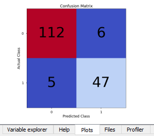
In classification we don’t use R-squared, but just the ratio of our correct predictions divided by all our predictions. We will look at the Confusion Matrix and the accuracy_score. And because our data is not perfectly balanced, we need to make sure our presicion_score, recall_score, and f1_score are also high. As we can see on the output below, we got a f1_score 90%, this is a good result!
y_pred_class=clf.predict(X_test)
y_pred_prob=clf.predict_proba(X_test)[:,1]

conf_matrix=confusion_matrix(y_test, y_pred_class)

# code for plotting the confusion matrix
plt.style.use('seaborn-poster')
plt.matshow(conf_matrix, cmap='coolwarm')
plt.gca().xaxis.tick_bottom()
plt.title('Confusion Matrix')
plt.ylabel('Actual Class')
plt.xlabel('Predicted Class')
for (i,j), corr_value in np.ndenumerate(conf_matrix):
    plt.text(j,i,corr_value,ha='center', va='center', fontsize=70)
plt.show()
OUTPUT:

accuracy_score(y_test, y_pred_class)

OUTPUT:
0.9352941176470588

precision_score(y_test, y_pred_class)

OUTPUT:
0.8867924528301887

recall_score(y_test, y_pred_class)

OUTPUT:
0.9038461538461539

f1_score(y_test, y_pred_class)

OUTPUT:
0.8952380952380953
Our Results
We have correctly classified all customers into two groups with low and high probability of signing up, in the future the company can contact only the second group and reduce marketing costs.
Which variables are important?
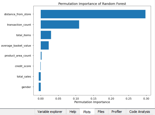
We are done, but we can use the results to do one more thing, answer the question which variables were important for the algorithm. The best method to use here is the method which uses permutation_importance.
result=permutation_importance(clf, X_test, y_test, n_repeats=10, random_state=42)

permutation_importance=pd.DataFrame(result['importances_mean'])
feature_names=pd.DataFrame(X.columns)
permutation_importance_summary=pd.concat([feature_names, permutation_importance], axis=1)
permutation_importance_summary.columns=['input_variable','permutation_importance']
permutation_importance_summary.sort_values(by='permutation_importance', inplace=True)# descending sorting

# plotting the results
plt.barh(permutation_importance_summary['input_variable'],permutation_importance_summary['permutation_importance'])
plt.title('Permutation Importance of Random Forest')
plt.xlabel('Permutation Importance')
plt.tight_layout()
plt.show()
OUTPUT:

Photo source: markus_winkler/Unsplash